[TOC]
1. Introduction
任务所要用到的文件
Files included in this exercise ex1.m - Octave/MATLAB script that steps you through the exercise ex1 multi.m - Octave/MATLAB script for the later parts of the exercise ex1data1.txt - Dataset for linear regression with one variable ex1data2.txt - Dataset for linear regression with multiple variables submit.m - Submission script that sends your solutions to our servers [?] warmUpExercise.m - Simple example function in Octave/MATLAB [?] plotData.m - Function to display the dataset [?] computeCost.m - Function to compute the cost of linear regression [?] gradientDescent.m - Function to run gradient descent [†] computeCostMulti.m - Cost function for multiple variables [†] gradientDescentMulti.m - Gradient descent for multiple variables [†] featureNormalize.m - Function to normalize features [†] normalEqn.m - Function to compute the normal equations ? indicates files you will need to complete † indicates optional exercises
2. Assignment
2.1 Simple Octave/MATLAB function
这一步很简单,在写好的函数内添加内容
打开warmUpExercise.m文件
function A = warmUpExercise()

% ============= YOUR CODE HERE ==============

% 在这里添加内容
A = eye(5);

% ===========================================

end
2.2 Linear regression with one variable
这一节有三个任务:
- 可视化数据
- 计算梯度下降
- 结果可视化
2.2.1 Plotting the Data
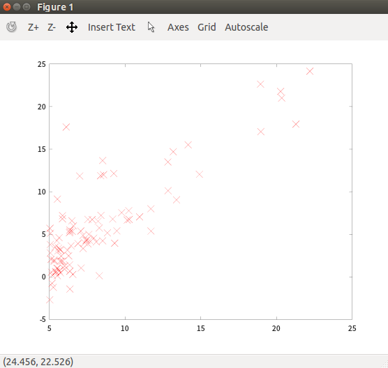
导入'ex1data1.txt 文件数据,然后显示
首先写一个显示数据的函数plotData 保存到文件plotData.m
function plotData(x, y)
figure; % open a new figure window

% ====================== YOUR CODE HERE ======================

plot(x, y, 'rx', 'MarkerSize', 10);
% marker
%      'x'  cross
% color
%      'r'  Red
% 用红色叉叉标记坐标点,标记大小为10
% ============================================================

end
plot使用
导入数据,调用函数plotData :
ex1data1.txt:
6.1101,17.592
5.5277,9.1302
8.5186,13.662
7.0032,11.854
5.8598,6.8233
...
data = load('ex1data1.txt');
X = data(:, 1); y = data(:, 2);
plotData(X, y);
结果展示:
2.2.2 Gradient Descent
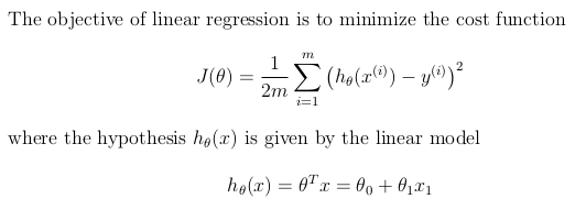
首先计算损失函数,公式如下:
代码文件computeCost.m
function J = computeCost(X, y, theta)

m = length(y); % number of training examples
J = 0;

% ====================== YOUR CODE HERE ======================

J = sum((X*theta -y).^2)/2/m;

% ============================================================
end
然后计算梯度下降,公式如下:
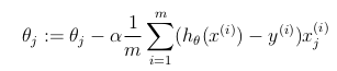
代码文件gradientDescent.m
function [theta, J_history] = gradientDescent(X, y, theta, alpha, num_iters)

m = length(y); % number of training examples
J_history = zeros(num_iters, 1);

for iter = 1:num_iters

    % ====================== YOUR CODE HERE ======================

theta = theta - (sum(alpha * (X*theta -y).*X)/m)';

    % ============================================================

    % Save the cost J in every iteration
    J_history(iter) = computeCost(X, y, theta);

end

end
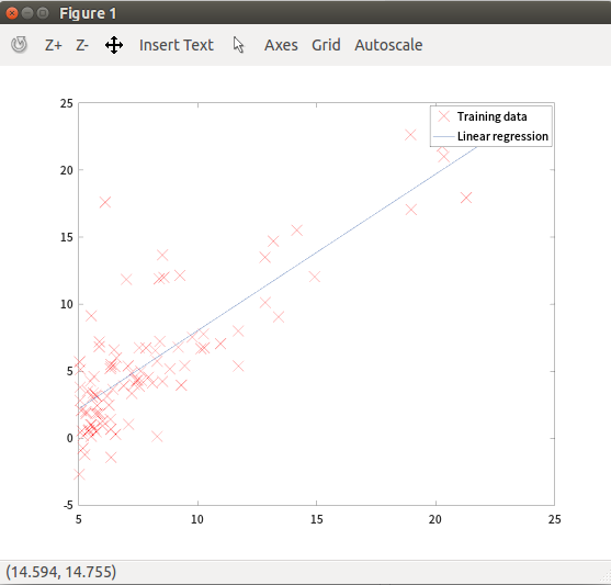
最后绘制回归曲线
theta = gradientDescent(X, y, theta, alpha, iterations);
hold on; % keep previous plot visible
plot(X(:,2), X*theta, '-')
legend('Training data', 'Linear regression')
hold off % don't overlay any more plots on this figure
legend 为每个绘制的数据序列创建一个带有描述性标签的图例。
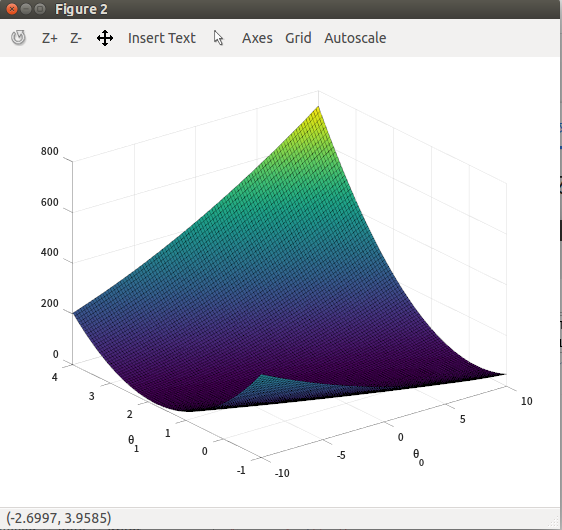
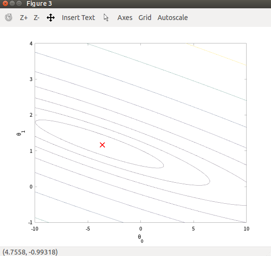
2.2.3 Visualizing J(θ)
损失值可视化,这部分不用自己写代码。首先通过linspace 取一些范围theta值。然后调用computeCost获取每一组theta值的cost。
% Grid over which we will calculate J
theta0_vals = linspace(-10, 10, 100);
theta1_vals = linspace(-1, 4, 100);

% initialize J_vals to a matrix of 0's
J_vals = zeros(length(theta0_vals), length(theta1_vals));

% Fill out J_vals
for i = 1:length(theta0_vals)
    for j = 1:length(theta1_vals)
	  t = [theta0_vals(i); theta1_vals(j)];
	  J_vals(i,j) = computeCost(X, y, t);
    end
end
获取到cost之后调用surf 函数画出来一个三维曲面图。代码如下:
% Because of the way meshgrids work in the surf command, we need to
% transpose J_vals before calling surf, or else the axes will be flipped
J_vals = J_vals';
% Surface plot
figure;
surf(theta0_vals, theta1_vals, J_vals)
xlabel('\theta_0'); ylabel('\theta_1');
% Contour plot
figure;
% Plot J_vals as 15 contours spaced logarithmically between 0.01 and 100
contour(theta0_vals, theta1_vals, J_vals, logspace(-2, 3, 20))
xlabel('\theta_0'); ylabel('\theta_1');
hold on;
plot(theta(1), theta(2), 'rx', 'MarkerSize', 10, 'LineWidth', 2);
% theta是通过前面计算出来的最优参数。
2.3 Linear regression with multiple variables
2.3.1 特征归一化(Feature Normalization)
代码文件featureNormalize.m
function [X_norm, mu, sigma] = featureNormalize(X)

% You need to set these values correctly
X_norm = X;
mu = zeros(1, size(X, 2));
sigma = zeros(1, size(X, 2));

% ====================== YOUR CODE HERE ======================

mu = mean(X);
sigma = std(X);
X_norm = (X - mu)./sigma;

% X_norm = (X - mean(X))./std(X);

% ============================================================

end
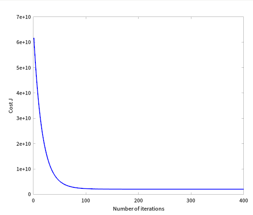
2.3.2 Gradient Descent
对于矩阵向量之间的计算多变量和单变量的公式都一样。所以computeCostMulti.m and gradientDescentMulti.m 两个文件代码请看前面。
绘制成本函数曲线:
% Choose some alpha value
alpha = 0.03;
num_iters = 400;

% Init Theta and Run Gradient Descent
theta = zeros(3, 1);
[theta, J_history] = gradientDescentMulti(X, y, theta, alpha, num_iters);

% Plot the convergence graph
figure;
plot(1:numel(J_history), J_history, '-b', 'LineWidth', 2);
xlabel('Number of iterations');
ylabel('Cost J');
2.3.3 Normal Equations
寻找最优参数theta,还可以通过正规方程实现,不用设置学习率α和特征缩放,也不用计算梯度下降,迭代至收敛。公式:

代码文件:normalEqn.m
function [theta] = normalEqn(X, y)

theta = zeros(size(X, 2), 1);

% ====================== YOUR CODE HERE ======================

theta = pinv(X'*X)*X'*y

% ============================================================

end
至此,作业1完成,Congratulation!