[TOC]
Octabe install
推荐 使用Octave安装包安装.
On Ubuntu, you can use:
sudo apt-get update && sudo apt-get install octave
On Fedora, you can use:
sudo yum install octave-forge
Octave 使用
GNU Octave, version 4.2.2
Copyright (C) 2018 John W. Eaton and others.
Octave was configured for "x86_64-pc-linux-gnu".
...
For more information, visit http://www.octave.org/get-involved.html

>> 1 ==2
ans = 0
>> 1~=2
ans = 1
# 9x9 随机 0~1
>> rand(9,9)
ans =

   0.3560386   0.4607871   0.8059847   0.2042094   0.2411058   0.9311803   0.8023873   0.8208079   0.9631931
   0.4604231   0.0222901   0.6693275   0.5887816   0.0076518   0.1670580   0.6335819   0.1711659   0.1405882
   0.0519485   0.3400714   0.2909762   0.3687556   0.7300303   0.3436051   0.1679526   0.2550348   0.0342722
   0.9379501   0.7760394   0.0859048   0.3292712   0.2385854   0.8567406   0.2433711   0.8027390   0.4103872
   0.8297066   0.5138018   0.3540072   0.7688630   0.7550758   0.0676738   0.3528168   0.5365513   0.8800598
   0.3350162   0.8376844   0.7863446   0.6448189   0.1355422   0.0235755   0.2975952   0.2879286   0.8854084
   0.2484960   0.2086548   0.4821656   0.5838678   0.2676164   0.8016253   0.5552146   0.2787187   0.7647289
   0.7559019   0.2639478   0.4199944   0.5312557   0.5202589   0.7852354   0.5681352   0.1088001   0.6572705
   0.9477478   0.4998028   0.4179308   0.0513819   0.8775790   0.5860457   0.3993368   0.3765168   0.2140254

>> ones(9,9)
ans =

   1   1   1   1   1   1   1   1   1
   1   1   1   1   1   1   1   1   1
   1   1   1   1   1   1   1   1   1
   1   1   1   1   1   1   1   1   1
   1   1   1   1   1   1   1   1   1
   1   1   1   1   1   1   1   1   1
   1   1   1   1   1   1   1   1   1
   1   1   1   1   1   1   1   1   1
   1   1   1   1   1   1   1   1   1

>> W = zeros(9,9);
>> W
W =

   0   0   0   0   0   0   0   0   0
   0   0   0   0   0   0   0   0   0
   0   0   0   0   0   0   0   0   0
   0   0   0   0   0   0   0   0   0
   0   0   0   0   0   0   0   0   0
   0   0   0   0   0   0   0   0   0
   0   0   0   0   0   0   0   0   0
   0   0   0   0   0   0   0   0   0
   0   0   0   0   0   0   0   0   0

>> rand(1, 2)
ans =
   0.76409   0.77792

>> sqrt(9)
ans =  3
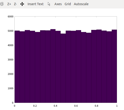
>> A = rand(1, 100000);
>> hist(A, 20)
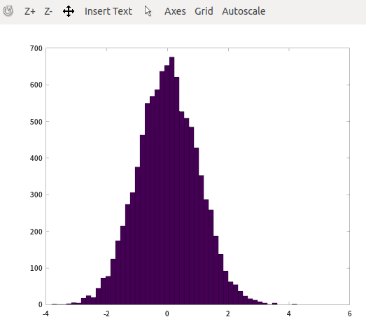
# 符合正太分布的随机数,randn,  u=0,seigema=1
>> A = randn (1,10000);
>> hist(A, 50)
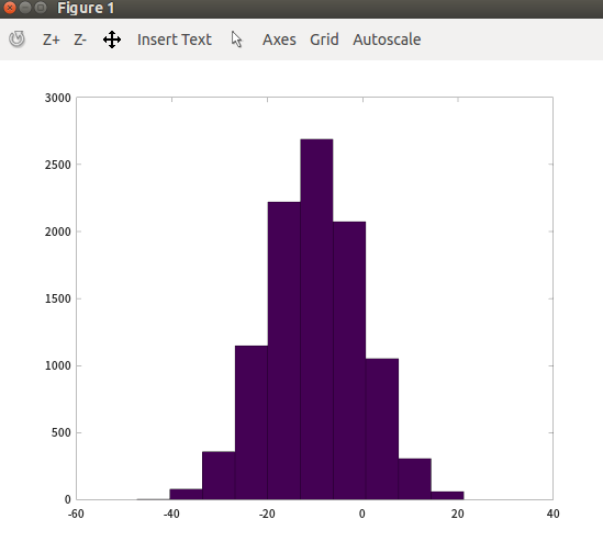
# u= -10 , segema = 98
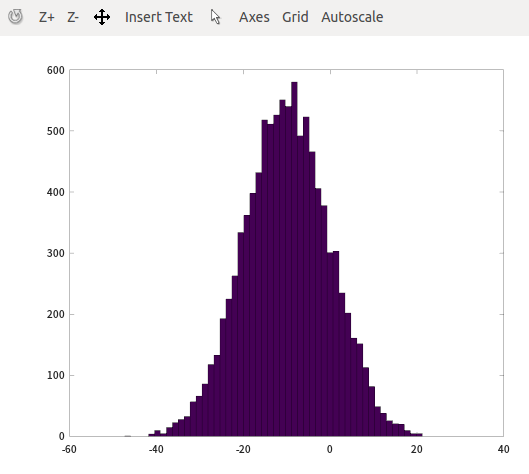
>> W = -10 + sqrt(98)*(randn(1,10000));
>> hist(W)
>> hist(W, 50)
>> eye(5)
ans =

Diagonal Matrix #单位矩阵

   1   0   0   0   0
   0   1   0   0   0
   0   0   1   0   0
   0   0   0   1   0
   0   0   0   0   1

>> size (W)
ans =

       1   10000

>> length (W)
ans =  10000
>> W = zeros (5)
W =

   0   0   0   0   0
   0   0   0   0   0
   0   0   0   0   0
   0   0   0   0   0
   0   0   0   0   0

>> length (W)
ans =  5

>> W = zeros (5, 4)
W =

   0   0   0   0
   0   0   0   0
   0   0   0   0
   0   0   0   0
   0   0   0   0

>> length (W)
ans =  5

>> W = zeros (2, 4)
W =

   0   0   0   0
   0   0   0   0

>> length (W)
ans =  4

# 注意,length 表示 航和列中,较大的这个
# length (W) = max (size (A))
octave还可以执行部分shell命令
>> pwd
ans = /home/alex/data_files/software/xmind/xmind-8-update8-linux/XMind_amd64
>> cd
>> pwd
ans = /home/alex
>> ls
2018-10-16 18-01-44

>> load sogou-qimpanel:0.pid

>> who
Variables in the current scope:

W    ans
举证其他表示方法
>> A = [1 2; 3 4; 5 6]
A =

   1   2
   3   4
   5   6

>> B = [11 12; 13 14; 15 16]
B =

   11   12
   13   14
   15   16

>> C = [A B]
C =

    1    2   11   12
    3    4   13   14
    5    6   15   16

>> D = [A; B]
D =

    1    2
    3    4
    5    6
   11   12
   13   14
   15   16

# transpose
>> D'
ans =

    1    3    5   11   13   15
    2    4    6   12   14   16

>> E = rand(5)
E =

   0.382889   0.826820   0.143657   0.105050   0.799284
   0.342433   0.729053   0.571096   0.498017   0.581522
   0.299401   0.346902   0.273341   0.138887   0.505162
   0.745145   0.132160   0.319004   0.978364   0.488847
   0.368702   0.029850   0.391279   0.496332   0.533725

>> E = rand(5,1)
E =

   0.99898
   0.63184
   0.95289
   0.37744
   0.91223
最大值
>> E = rand(1,10)
E =

   0.790997   0.471432   0.598649   0.593467   0.342134   0.960598   0.752763   0.021469   0.271880   0.111108

>> max (E)
ans =  0.96060
>> [value, index] = max(E)
value =  0.96060
index =  6
过滤筛选
>> E < 0.5
ans =

  0  1  0  0  1  0  0  1  1  1

>> find(E < 0.5)
ans =

    2    5    8    9   10

>> E
E =

   0.790997   0.471432   0.598649   0.593467   0.342134   0.960598   0.752763   0.021469   0.271880   0.111108

>> [value, index] = find(E<0.5)
value =

   1   1   1   1   1

index =

    2    5    8    9   10

>> E = rand(5,5)
E =

   0.787163   0.617232   0.703976   0.436314   0.410497
   0.440223   0.812849   0.242780   0.869555   0.278506
   0.240996   0.931844   0.060643   0.612793   0.227300
   0.451394   0.673056   0.184734   0.143215   0.803382
   0.795615   0.979938   0.857430   0.963706   0.765059

>> [value, index] = find(E<0.5)
value =

   2
   3
   4
   2
   3
   4
   1
   4
   1
   2
   3

index =

   1
   1
   1
   3
   3
   3
   4
   4
   5
   5
   5

>> [rows, colums] = find(E<0.5)
rows =

   2
   3
   4
   2
   3
   4
   1
   4
   1
   2
   3

colums =

   1
   1
   1
   3
   3
   3
   4
   4
   5
   5
   5
相关计算
>> sum(E)
ans =

   2.9953   2.4057   2.3705   3.2331   2.2077

>> prod(E)
ans =

   0.0337328   0.0098164   0.0058173   0.0925647   0.0138977

>> floor (E)
ans =

   0   0   0   0   0
   0   0   0   0   0
   0   0   0   0   0
   0   0   0   0   0
   0   0   0   0   0

>> ceil (E)
ans =

   1   1   1   1   1
   1   1   1   1   1
   1   1   1   1   1
   1   1   1   1   1
   1   1   1   1   1

>> F = randn (5)
F =

   1.73542  -0.97333   0.90465   0.28529   1.89615
  -0.56606  -0.78233  -1.20289   0.77386   0.64770
  -1.54203   0.49252   1.34071   1.56246  -1.48515
  -1.82310  -1.68507   1.41672  -1.24164  -0.20081
   1.12516   0.63253  -1.90412  -1.23104   0.66748

>> ceil (F)
ans =

   2  -0   1   1   2
  -0  -0  -1   1   1
  -1   1   2   2  -1
  -1  -1   2  -1  -0
   2   1  -1  -1   1

>> floor (F)
ans =

   1  -1   0   0   1
  -1  -1  -2   0   0
  -2   0   1   1  -2
  -2  -2   1  -2  -1
   1   0  -2  -2   0

>> prod(F)
ans =

  -3.10731  -0.39973   3.93571   0.52725   0.24448

>> sum(F)
ans =

  -1.07060  -2.31567   0.55507   0.14892   1.52537

>> G1 = rand(3)
G1 =

   0.536005   0.039219   0.756845
   0.378762   0.097467   0.124591
   0.567407   0.395335   0.371280

>> G2 = rand(3)
G2 =

   0.210937   0.263702   0.241626
   0.191786   0.871084   0.903337
   0.350747   0.768891   0.047243

>> max(G1,G2)
ans =

   0.53601   0.26370   0.75684
   0.37876   0.87108   0.90334
   0.56741   0.76889   0.37128

>> max(G1)
ans =

   0.56741   0.39533   0.75684

>> max(G1, [], 1)
ans =

   0.56741   0.39533   0.75684

>> max(G1, [], 2)
ans =

   0.75684
   0.37876
   0.56741

>> max(max(G1))
ans =  0.75684
>> max(G1(:))
ans =  0.75684
>> G1(:)
ans =

   0.536005
   0.378762
   0.567407
   0.039219
   0.097467
   0.395335
   0.756845
   0.124591
   0.371280

>> A
A =

   1   2
   3   4
   5   6
magic使用
>> magic (9)
ans =

   47   58   69   80    1   12   23   34   45
   57   68   79    9   11   22   33   44   46
   67   78    8   10   21   32   43   54   56
   77    7   18   20   31   42   53   55   66
    6   17   19   30   41   52   63   65   76
   16   27   29   40   51   62   64   75    5
   26   28   39   50   61   72   74    4   15
   36   38   49   60   71   73    3   14   25
   37   48   59   70   81    2   13   24   35

>> eye (9)
ans =

Diagonal Matrix

   1   0   0   0   0   0   0   0   0
   0   1   0   0   0   0   0   0   0
   0   0   1   0   0   0   0   0   0
   0   0   0   1   0   0   0   0   0
   0   0   0   0   1   0   0   0   0
   0   0   0   0   0   1   0   0   0
   0   0   0   0   0   0   1   0   0
   0   0   0   0   0   0   0   1   0
   0   0   0   0   0   0   0   0   1

>> magic (9) .* eye (9)
ans =

   47    0    0    0    0    0    0    0    0
    0   68    0    0    0    0    0    0    0
    0    0    8    0    0    0    0    0    0
    0    0    0   20    0    0    0    0    0
    0    0    0    0   41    0    0    0    0
    0    0    0    0    0   62    0    0    0
    0    0    0    0    0    0   74    0    0
    0    0    0    0    0    0    0   14    0
    0    0    0    0    0    0    0    0   35

>> sum(sum(magic (9) .* eye(9)))
ans =  369
>> sum(magic (9) .* eye(9))
ans =

   47   68    8   20   41   62   74   14   35
逆矩阵和转置
inverse and transport
# θ = ( X^T X )^−1 X^T y
# theta = pinv(X'*X)*X'*y
# inv pinv, pinv 可以处理逆矩阵不是线性相关的问题。
>>  A
A =

   30   39   48    1   10   19   28
   38   47    7    9   18   27   29
   46    6    8   17   26   35   37
    5   14   16   25   34   36   45
   13   15   24   33   42   44    4
   21   23   32   41   43    3   12
   22   31   40   49    2   11   20

>> pinv(A)
ans =

   8.1633e-04   8.1633e-04   2.1165e-02  -1.9533e-02  -2.0907e-03   4.1386e-03   4.0104e-04
  -2.0907e-03   2.4072e-02  -1.9533e-02   1.2316e-03   4.0104e-04   8.1633e-04   8.1633e-04
   2.1165e-02  -1.9117e-02   4.0104e-04  -2.0907e-03   3.7233e-03   8.1633e-04   8.1633e-04
  -1.7041e-02   8.1633e-04   8.1633e-04   8.1633e-04   8.1633e-04   8.1633e-04   1.8673e-02
   8.1633e-04   8.1633e-04  -2.0907e-03   3.7233e-03   1.2316e-03   2.0750e-02  -1.9533e-02
   8.1633e-04   8.1633e-04   1.2316e-03   4.0104e-04   2.1165e-02  -2.2439e-02   3.7233e-03
   1.2316e-03  -2.5059e-03   3.7233e-03   2.1165e-02  -1.9533e-02   8.1633e-04   8.1633e-04

>> A * pinv(A)
ans =

   1.0000e+00  -4.5103e-17  -1.5266e-16  -1.0408e-15  -4.4409e-16   5.5338e-16   7.6675e-16
  -7.0907e-16   1.0000e+00   4.7878e-16   2.4633e-16   2.4980e-16   4.2067e-17  -7.4853e-16
   7.4463e-16  -1.4485e-16   1.0000e+00  -8.9165e-16   2.4980e-16   1.1493e-16   4.3455e-16
  -3.3437e-16   5.2822e-16  -4.3715e-16   1.0000e+00   2.7756e-17   1.6697e-16  -6.5052e-17
  -1.2317e-16   2.1684e-16  -1.8908e-16  -5.9674e-16   1.0000e+00   2.5847e-16   9.9053e-16
  -6.6787e-16  -3.0878e-16   1.0270e-15   6.9389e-17  -2.7756e-17   1.0000e+00  -5.2042e-16
  -5.9501e-16   1.0408e-17   4.8572e-16  -1.3878e-17   3.3307e-16  -1.9082e-17   1.0000e+00
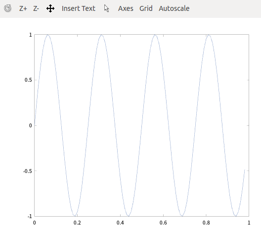
画图
>> t=[0:0.01:0.98];
>> y1=sin(2*pi*4*t);
>> plot(t,y1);
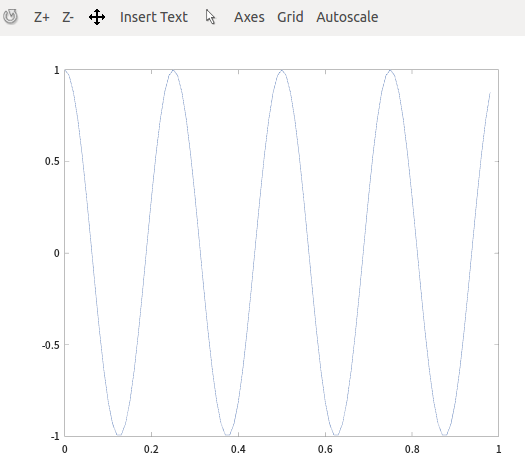
>> y2=cos(2*pi*4*t);
>> plot(t,y2)
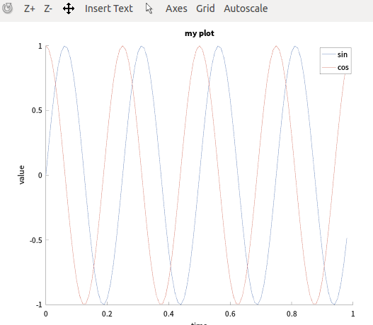
一个图,多个曲线
>> t=[0:0.01:0.98];
>> y1=sin(2*pi*4*t);
>> y2=cos(2*pi*4*t);
>> hold on; #保持上图
>> plot(t,y1);
>> plot(t,y2)
>> xlabel ('time')
>> ylabel ('value')
# 图例线
>> legend('sin', 'cos')
>> title('my plot')
# 导出
>> cd
>> print -dpng 'myplot.png'
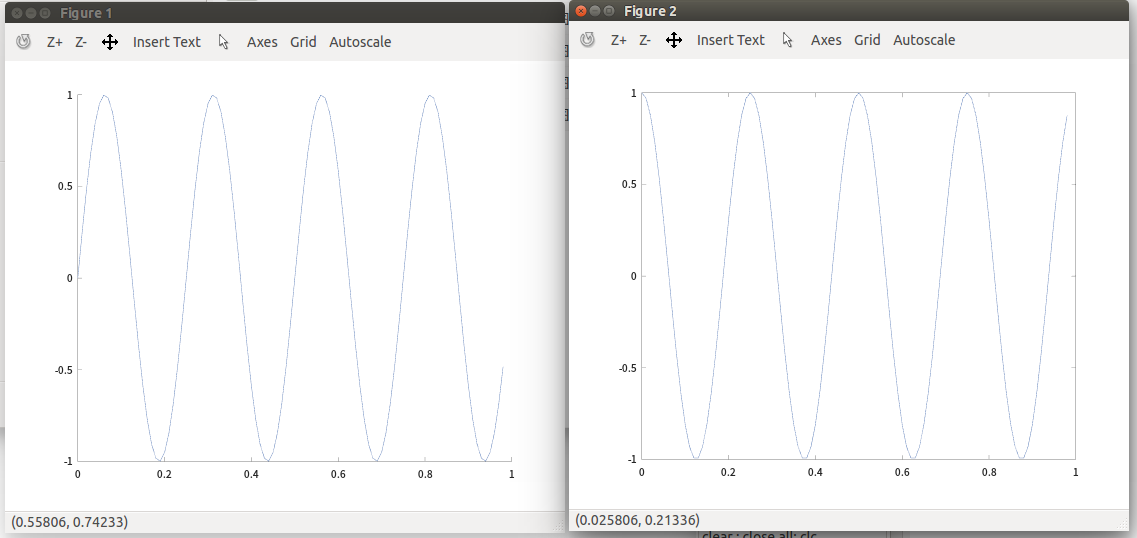
多个figure同时呈现
>> t=[0:0.01:0.98];
>> y1=sin(2*pi*4*t);
>> y2=cos(2*pi*4*t);
>> hold on;
>> figure (1);plot(t,y1);
>> figure (2);plot(t,y2);
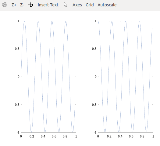
子图显示
>> subplot (1,2,1);
>> plot(t,y1);
>> subplot (1,2,2);
>> plot(t,y2);
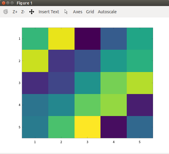
imagesc
>> imagesc (magic (5))
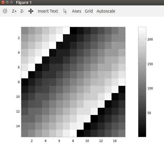
>> imagesc (magic (15)), colorbar, colormap gray;
>> help imagesc
'imagesc' is a function from the file /usr/share/octave/4.2.2/m/image/imagesc.m
-- imagesc (IMG)
-- imagesc (X, Y, IMG)
-- imagesc (..., CLIMITS)
-- imagesc (..., "PROP", VAL, ...)
-- imagesc ("PROP1", VAL1, ...)
-- imagesc (HAX, ...)
-- H = imagesc (...)
Display a scaled version of the matrix IMG as a color image.
>> for i=1:10, v(i)=2^i; end;
>> v
v =

      2      4      8     16     32     64    128    256    512   1024

>> include=1:10;
>> for i=include , disp(i); end;
 1
 2
 3
 4
 5
 6
 7
 8
 9
 10
>> i=1; while i<=5. v(i) = 100; i=i+1; end
>> v
v =

    100    100    100    100    100     64    128    256    512   1024

>> while true,
v(i) = 999;
if i ==7, break;
end; end;
>> v
v =

    100    100    100    100    100    999    999    256    512   1024

>> i = 1;
>> while true,
v(i) = 999;
i = i+ 1;
if i ==7, break;
end; end;
>> v
v =

    999    999    999    999    999    999    999    256    512   1024

>> x = 2; if x ==1 , disp('the value is one');
elseif x == 2, disp('the value is two');
else disp('the value is not one or two');
end;
好啦,有这些基础就够用啦。再加上有help的帮助,遇到上面问题就知道怎么找解决办法了。